Scalability Deep Dive: Capacity Planning & Back-of-Envelope Math

You Scaled. Now What?

In the Scalability post, we covered the big picture: vertical vs horizontal scaling, stateless architecture, and the classic traps. If you haven't read it, start there.

But here's what that post didn't answer: how many servers do you actually need?

Not it depends. Not start small and scale. A real number, with real reasoning behind it. That's what separates an engineer who understands scalability concepts from one who can actually plan and defend an infrastructure decision in a production environment.

This post is about the math.

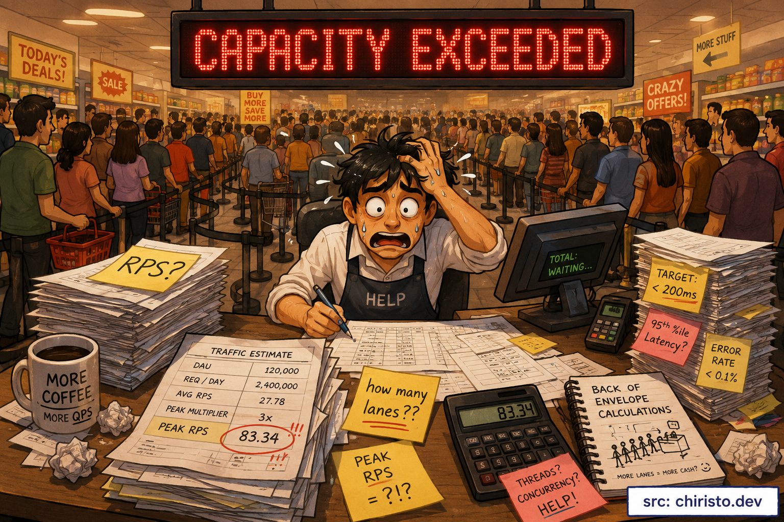
The Question Most Engineers Can't Actually Answer

Ask a senior engineer "how do you know when you need more servers?" and they'll say: when CPU hits 70%, when latency spikes, when the dashboard turns red.

That's reactive scaling. You're responding to the fire, not preventing it.

Ask them before the traffic spike: how many servers will you need to handle 50,000 requests per second? - and most will pause. Because that question requires actual numbers, and most systems aren't designed with those numbers written down anywhere.

Capacity planning is the practice of answering that question before the system is under load. It's not about being exactly right. It's about being close enough to make safe decisions and wrong in the right direction (over-provisioned, not under).

Back-of-Envelope Math: The Core Skill

Back-of-envelope estimation is a structured way to get to a reasonable number fast. The goal is not precision. The goal is the right order of magnitude with justifiable assumptions.

Here's the framework:

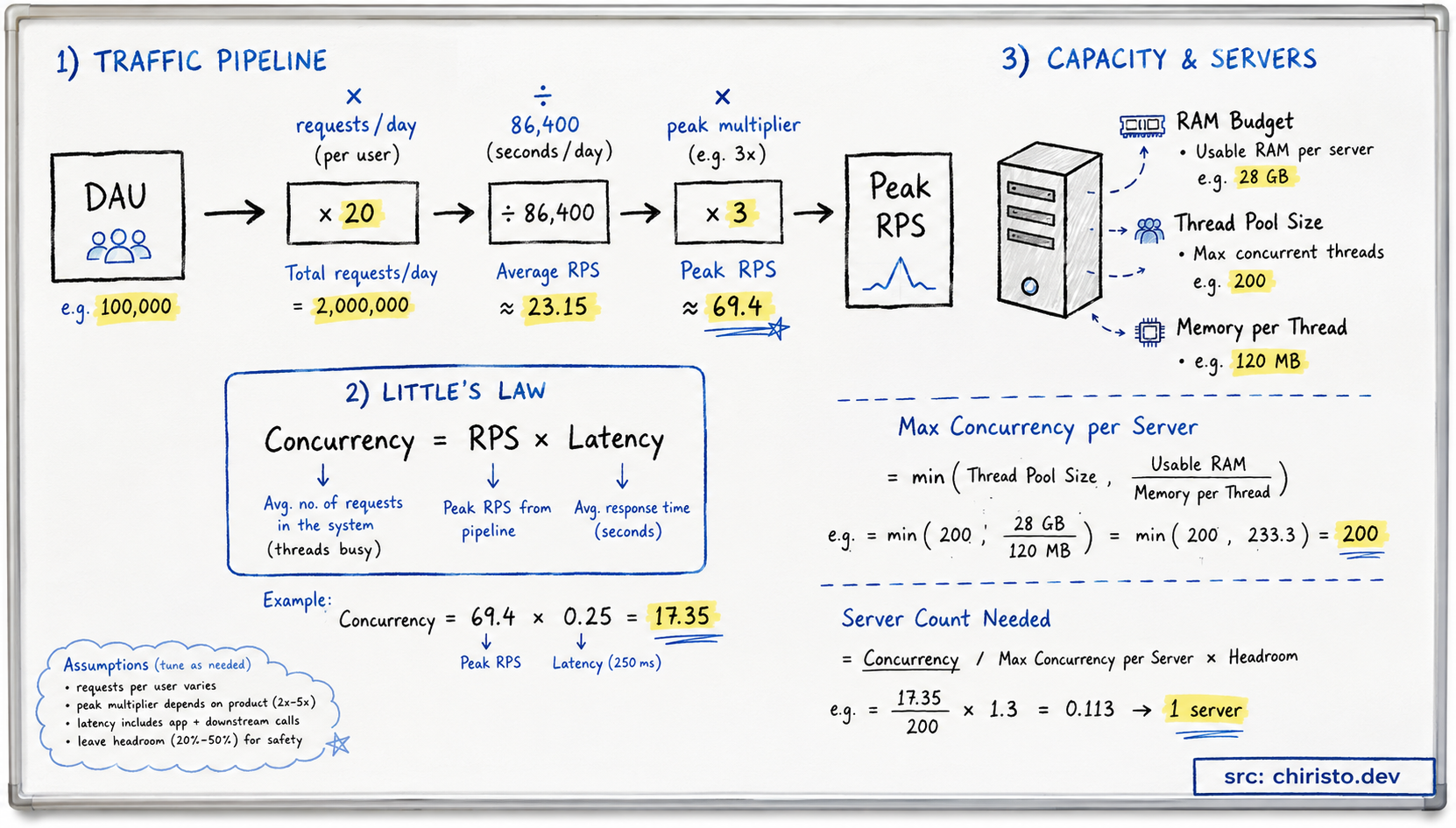
Step 1: Establish Your RPS (Requests Per Second)

Start with daily active users (DAU) and your read/write ratio.

DAU = 10,000,000 users
Average requests per user per day = 20
Total daily requests = 200,000,000

Seconds in a day = 86,400
Average RPS = 200,000,000 / 86,400 ≈ 2,315 RPS

But you never plan for average. You plan for peak. Real traffic follows a wave pattern — dead at 3am, brutal at 9am and 8pm. A common safe multiplier for consumer apps is 3x to 5x average RPS for peak.

Peak RPS = 2,315 × 4 = ~9,260 RPS

That's your planning number.

Step 2: Estimate Memory Per Request

A single server has a fixed amount of RAM. How much does each active request consume?

This depends on your stack, but a realistic breakdown for a typical API server:

Per-request heap allocation:     ~50 KB  (JSON parsing, response objects)
Thread or goroutine stack:       ~8 KB   (Go) to ~1 MB (Java thread)
Connection overhead:             ~4 KB   (TCP buffer)
Session / context data:          ~10 KB

Conservative total: ~70-100 KB per concurrent request

If your server has 16 GB RAM and you reserve 4 GB for the OS and runtime:

Available RAM = 12 GB = 12,288 MB
Memory per request = 100 KB = 0.1 MB
Max concurrent requests = 12,288 / 0.1 = ~122,880

That's a ceiling, not a target. Running at 80% capacity is a safer operating point.

Safe concurrent requests per server = ~98,000

Step 3: Factor in Latency Budget

Concurrent requests != RPS directly. You need to account for how long each request holds a thread or connection alive.

This is Little's Law:

Concurrency = RPS × Average Latency (in seconds)

If average latency = 50ms = 0.05s:
Concurrency = 9,260 RPS × 0.05 = 463 concurrent requests per second

So a single 16 GB server can theoretically handle far more than 9,260 RPS from a memory standpoint, but your thread pool and I/O limits will constrain it long before RAM does.

Step 4: Thread Pool Math

Most blocking I/O servers (Java, Python, Node.js with sync calls) have a thread pool that limits actual concurrency.

Thread pool size = 500 threads (typical)
Each thread handles 1 blocking request at a time
Max throughput = 500 threads / 0.05s latency = 10,000 RPS per server

For async/non-blocking servers (Go, Node.js with async), threads aren't the bottleneck — event loop saturation and I/O wait are. But the principle of finding your real ceiling before RAM applies the same way.

Server count for 9,260 peak RPS:
= Peak RPS / Max RPS per server
= 9,260 / 10,000
= ~1 server (theoretically)

You never run on one server. Add redundancy, headroom for GC pauses, and rolling deployment capacity:

Recommended minimum = 3 servers (1 spare + 1 for rolling deploys + 1 active)
Realistic production = 5-6 servers for this load profile

Read vs. Write: Why Symmetric Planning Fails

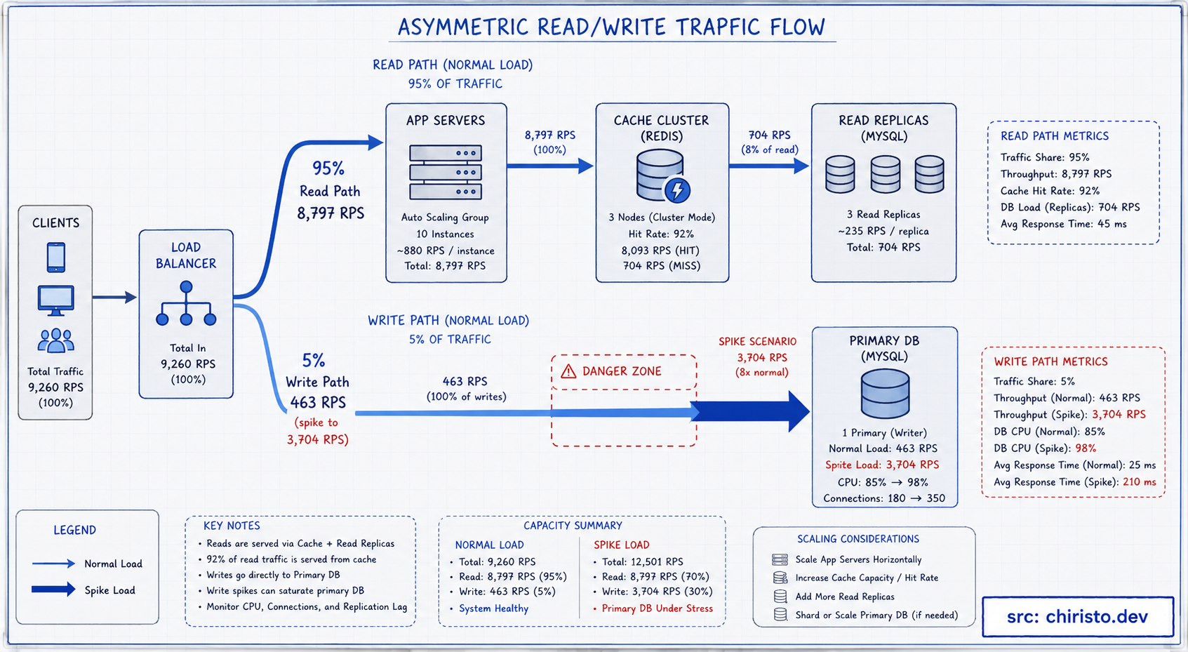
Most systems aren't balanced. They're heavily read-dominant. A typical social feed: 95% reads, 5% writes. An analytics platform might flip that. Getting this ratio wrong in your planning means you over-provision the wrong tier entirely.

The Read/Write Breakdown

For a read-heavy app at 9,260 peak RPS:

Read RPS  = 9,260 × 0.95 = 8,797 RPS  -> hits your cache + read replicas
Write RPS = 9,260 × 0.05 = 463 RPS    -> hits your primary DB / write path

Reads are cheap if you have a cache in front. Writes are expensive: they hit the primary, trigger replication lag, and may invalidate cache entries.

Your infrastructure split should reflect this:

• Read path: horizontally scalable app servers + cache cluster + read replicas
• Write path: smaller, more reliable primary DB cluster with strict latency SLAs

Peak Multipliers Are Not Symmetric Either

Traffic spikes aren't uniform across read and write paths. A flash sale causes a write spike (orders). A breaking news event causes a read spike (page views). Plan peak multipliers separately per path, not just on overall RPS.

Read peak multiplier:  4x  -> 35,188 read RPS
Write peak multiplier: 8x  -> 3,704 write RPS (flash sale scenario)

That write spike of 8x against a primary database that was sized for 463 RPS is where systems go down.

The Hidden Variables the Math Doesn't Catch

The calculations above will get you in the right ballpark. But production systems fail for reasons that don't show up in a spreadsheet.

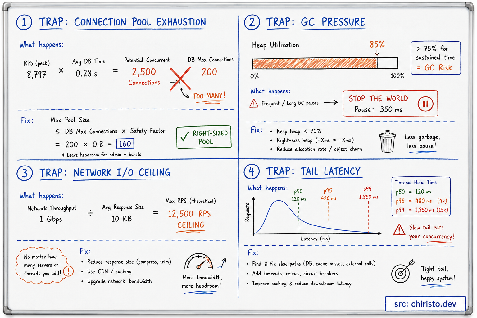
1. Connection Pool Exhaustion

Your app server can handle 10,000 RPS, but your database accepts 200 connections max. At scale, if each app server thread opens its own DB connection, you exhaust the pool and requests queue up - or crash.

DB max connections = 200
App servers = 5, threads per server = 500
Total potential connections = 2,500 → 12.5× over DB limit

Fix: connection pooling (PgBouncer, HikariCP). Size your pool per server, not per thread.

Pool size per server = DB max connections / number of app servers
= 200 / 5 = 40 connections per server

This is one of the most common capacity planning oversights in real systems.

2. GC Pressure at Load

Java and JVM-based systems have stop-the-world GC pauses. At low load, these are invisible. At peak load with heap pressure, a GC pause of 200-500ms turns your 50ms latency SLA into a cascade of timeout failures - because during that pause, requests queue up and the backlog compounds.

Capacity planning for JVM systems must include headroom for GC: never plan to operate above 60-65% heap utilization under peak load.

3. Network I/O Ceiling

CPU and RAM get all the attention. Network bandwidth is often the silent bottleneck. A server with a 1 Gbps NIC:

1 Gbps = 125 MB/s
Average response size = 10 KB
Max throughput = 125,000 KB/s / 10 KB = 12,500 RPS — network bound

If your response payloads are large (images, large JSON blobs), your server runs out of network before it runs out of CPU or RAM. Compression (gzip, brotli) and CDN offloading for static content are capacity tools, not just performance tools.

4. Tail Latency Skews Everything

You optimized for p50 latency (median). But your thread pool is sized for average behavior. At peak load, p99 latency (the slowest 1% of requests) might be 10x your average. Those slow requests hold threads and connections longer, reducing effective throughput below what your math predicted.

Always capacity plan against p95 or p99 latency, not p50.

When the Math Was Right and the System Still Failed

The Case of Friendster (2003-2009)

Friendster was the social network before MySpace, before Facebook. At its peak it had 115 million registered users. It didn't die from a lack of users. It died because it couldn't serve them.

Their core problem: every profile page required traversing a social graph - friends of friends of friends - with no caching layer and no read/write separation. Every page load triggered dozens of database queries on a schema that wasn't designed for graph traversal at scale.

The engineering team knew they had a traffic problem. The math wasn't wrong. But the math was being applied to the wrong bottleneck. They kept adding application servers while the database - a single monolithic relational schema performing graph queries - was the actual ceiling.

The lesson: capacity planning math is only as good as the bottleneck you're modeling. If you're planning app server capacity but the constraint is your database query pattern, more servers don't help. Find the actual bottleneck first, then apply the math.

The Prime Day Pattern

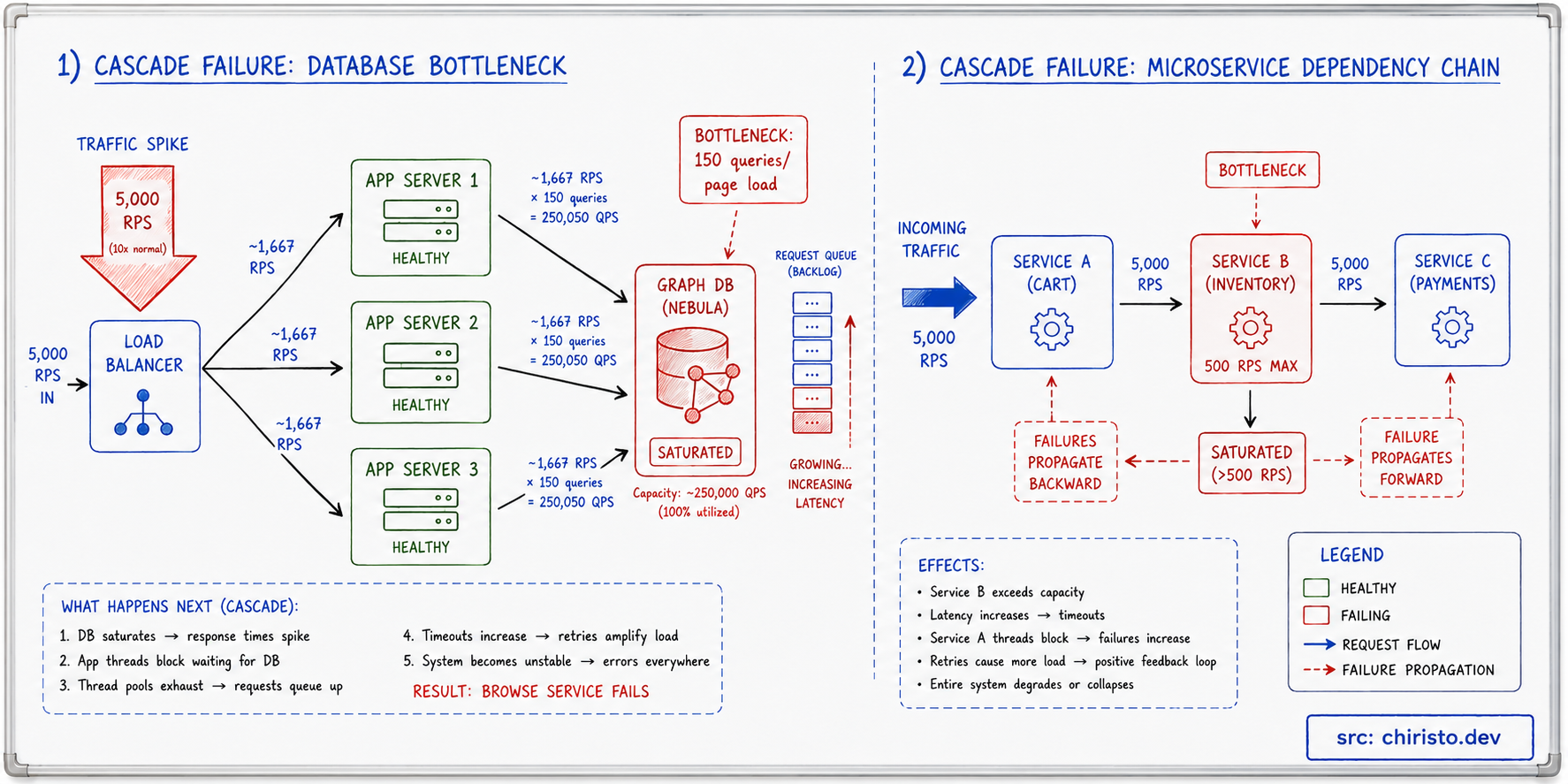
Amazon Prime Day 2018 saw Amazon's own website go down in some regions within the first hour. This wasn't a capacity math failure - Amazon has the best capacity planning teams on the planet. It was a dependency failure: third-party services and internal microservices that weren't included in the load testing scope hit their limits, and failures cascaded upstream.

The lesson: your capacity plan must include every dependency in the critical path, not just your own servers. A microservice you call that's sized for 500 RPS becomes your system's ceiling if you're sending it 5,000 RPS during peak.

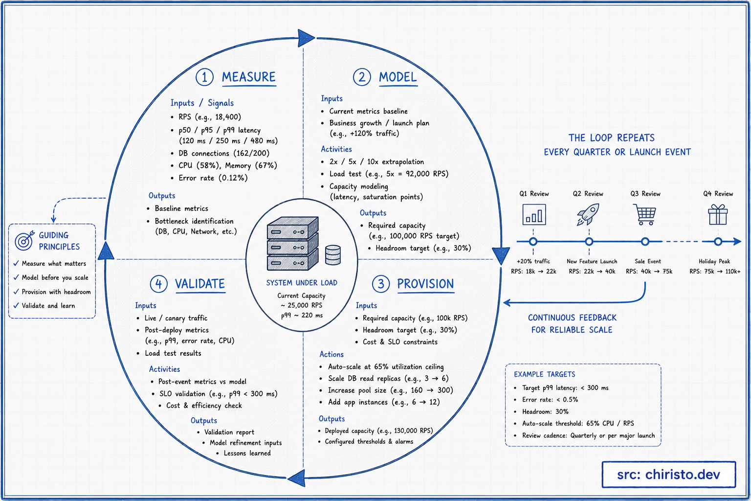
The Capacity Planning Feedback Loop

Good capacity planning isn't a one-time calculation before launch. It's a continuous loop tied to your observability stack.

The loop works like this:

Measure (what is the system actually doing right now?)

• RPS per service, p50/p95/p99 latency, error rate, CPU/RAM/network utilization, DB connection pool usage, queue depths

Model (what will the system need to do at 2x, 5x, 10x current load?)

• Extrapolate from current baselines using the math above
• Run load tests against your model assumptions

Provision (act on the model before you need to)

• Set auto-scaling thresholds below your calculated ceiling, not at it
• Common rule: scale out at 60-70% of your modeled ceiling to leave room for latency spikes and GC

Validate (did the provision match the reality?)

• After each load event (launch, campaign, prime day), compare actual metrics to modeled predictions
• Update your model with what you learned

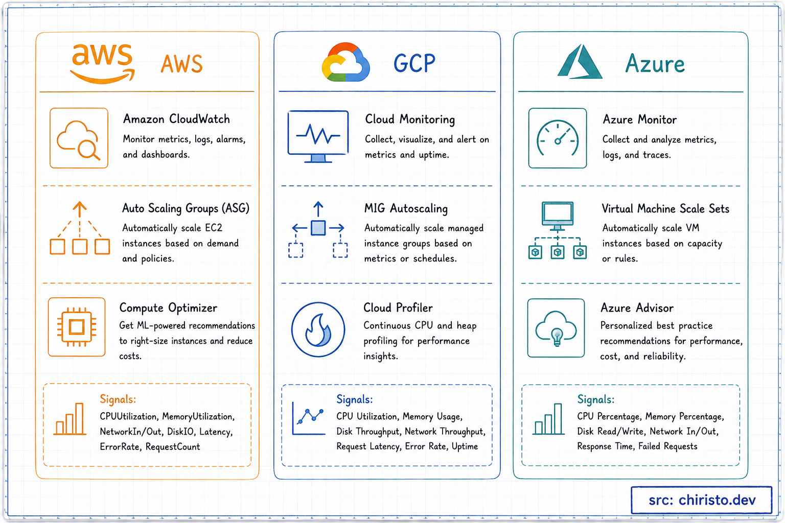
Cloud Provider Capacity Signals

The math above is cloud-agnostic. Here's how each major cloud surfaces these signals:

AWS:

• CloudWatch metrics: CPU, NetworkIn/Out, RequestCount per target (ALB), DB connections (RDS)
• Auto Scaling Groups with target tracking policies (scale at X% CPU or X requests per target)
• AWS Compute Optimizer: recommends right-sizing based on actual utilization history
• Trusted Advisor: flags underutilized or over-provisioned instances

GCP:

• Cloud Monitoring: custom metrics, uptime checks, latency percentile dashboards
• Managed Instance Groups with autoscaling on CPU, HTTP load balancing serving capacity, or custom Stackdriver metrics
• Cloud Profiler: identifies where CPU time is actually going so your math is modeling the right bottleneck

Azure:

• Azure Monitor + Application Insights: end-to-end latency tracking, dependency mapping for microservices
• VM Scale Sets with autoscale rules on CPU, memory, or custom metrics via Azure Monitor
• Azure Advisor: cost + performance recommendations based on usage patterns

The key difference: none of these tools do capacity planning for you. They give you the measurement layer. The modeling and provisioning decisions still require the math.

Quick Recap

Here's what you should be able to do now that you couldn't before reading this:

• Calculate peak RPS from DAU using a peak multiplier (never plan for average)
• Apply Little's Law to translate RPS + latency into concurrency requirements
• Run thread pool math to find your per-server throughput ceiling
• Separate read and write load with asymmetric peak multipliers
• Identify the four hidden bottlenecks: connection pool exhaustion, GC pressure, network I/O ceiling, tail latency
• Build a capacity planning feedback loop tied to your observability stack

The math is not hard. The discipline of actually doing it before the traffic spike is what separates good systems from the ones you read about in postmortems.

What's Next

This is one piece of the scalability picture. Knowing how many servers you need is only useful if you can distribute load across them intelligently - and if your data layer can keep up.

Next in the Scalability Deep Dive series: Sharding, Partitioning & Consistent Hashing. How do you split your data across nodes? What happens when a node goes down? Why does naive sharding cause hotspots, and how does a hash ring solve it?

The math gets spicier. See you there.